

2023 and Beyond: Industry Overview and Regulatory Environment
From 2020 to 2022, the maritime landscape has been significantly impacted: in particular, regulatory mandates have necessitated that ports and shipping lines actively review their operations to optimise the supply chain as a whole and adhere to the new environmental, social and governance (ESG) requirements.
Recognising the need for climate action, the IMO has mandated targets of carbon intensity reduction of 40% by 2030 and 70% by 2050, complemented by a minimum absolute reduction of 50% by 2050.
Port congestion is on the rise. Additionally, vessels want to arrive at a specific time and minimize alongside time to optimize and reduce the costs of shoreside labour, pilots, tugs, etc. Ports thus need to optimise berth scheduling, start to sequence vessels well in advance and also be mindful of greenhouse gas emissions (GHG). Shipping lines also need to comply with reduction of greenhouse gas emissions and fuel consumptions; their focus thus turns towards Just in Time (JIT) arrival.
Ports need to optimise berth scheduling, vessel sequencing and comply with green mandates. Shipping lines also need to comply with emission reduction targets.
The Solution: OCIANA™
A digital model to simulate the sequence of port operations (arrivals and departures) and assess the outcomes of each scenario, provides the capability to optimise the allocation of resources such as pilots, tugs and berths. This is essential to maximizing efficiency and meeting regulatory requirements.
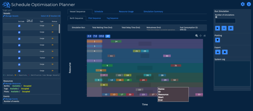
With OCIANA’s Schedule Optimisation Planner (SOP), port and terminal operators can explore and select the optimal sequence of operations that must be processed, and allocate the necessary resources accordingly.
How the Schedule Optimisation Planner (SOP) works:
- Port operations include the acquisition and release of seaside resources: berths, pilot vessels, and tugs. Based on GSTS’ work with port and pilotage authorities we were able to define the process for a vessel acquiring each resource to build a representative simulation model of the port.
- The Schedule Optimisation Planner (SOP) uses long-term vessel arrival forecasting, berth detection, and user inputs to build simulated scenarios to determine the optimal sequences of port operations.
- The simulation is run multiple times using different permutations of resource usage and sequencing. The simulations are then ranked on how well they meet the defined KPIs of lower wait time, lower delay time, and increased robustness (i.e., flexibility, or ability to withstand fluctuations).
- With the aid of the simulated sequences, operational planners can use the SOP to increase the efficiency of port operations, which will contribute significantly to a reduction in wait times and greenhouse gas emissions in real world scenarios.
Model Evaluation
GSTS’s engagement with The Port compares actual historical wait times and GHG emissions to those that would have resulted from the use of the SOP. Although the SOP will optimize reductions in delay times for departing vessels, the analysis focused on wait times because it was more feasible to determine actual vessel wait times as opposed to actual vessel delays, due to lack of planned departure information.
Comparison of simulated and actual wait times of an actual vessel voyage are presented in Figure 1. The average per vessel wait time in the simulation was 15.09 hours, whereas the average actual per vessel wait time was 32.68 hours – more than double that of the simulated. Also, noteworthy is that the actual wait times range much further than the simulated. The results also reveal that a small amount of wait time for most vessels may allow for a greater reduction of overall wait times. Average delay time for the simulation was 0.07 hours, which is far lower than the actual average wait time, indicating that most of the bottleneck at The Port is the result of time spent idling at anchor.
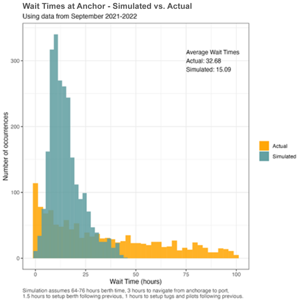
Figure 1: Distribution of average per vessel wait time at The Port for Actual (orange) vs. Simulated (green)
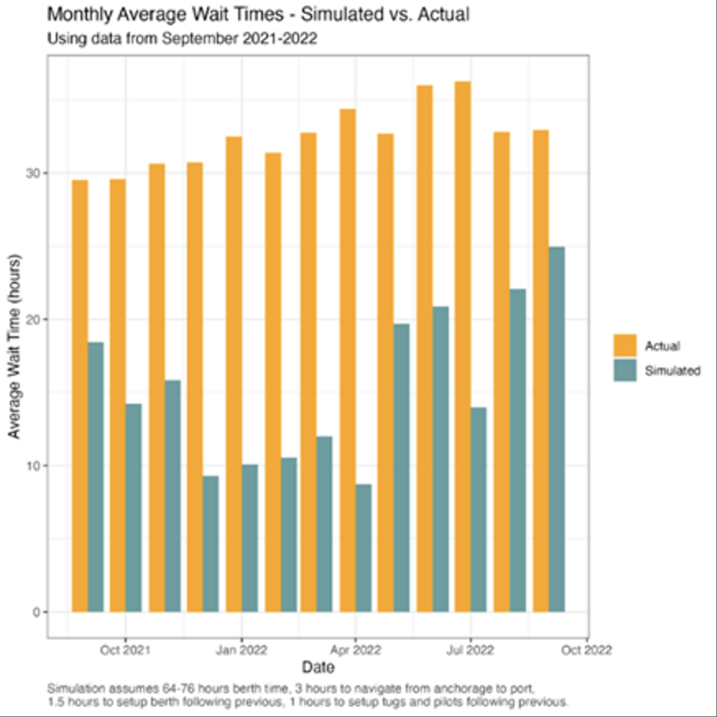
Figure 2: Average per vessel wait times for each month from September 2021-2022 for Actual (orange) vs. Simulated (green)
Monthly average wait times are shown in Figure 2, showing that SOP wait times are lower on average for each month. There is a striking decrease during the winter months when traffic tends to be lower.
We obtained greenhouse gas emission (GHG) estimates per vessel per week using the total wait time of the vessel and its fuel characteristics, which included the engine type and age, fuel type, and service speed of the vessel; all of which we obtained using IHS data. In cases where a vessel was partially or completely missing relevant IHS data we inputted the missing values with the average for the corresponding type of ship. Estimated GHG emissions between the two scenarios are shown in Figure 3. We see a substantial reduction in estimated GHG with the SOP with an average of 17.17 tonnes per vessel compared to the actual 70.83 tonnes per vessel.
These analyses suggest that the SOP can reduce wait times and associated GHG emissions by approximately 75%. However, it is possible that emissions can be further reduced (and on a much larger scale) by incorporating the concept of Just-In-Time arrivals (JIT). For instance, if we know that a vessel will have to incur waiting time, the vessel can reduce its speed (and associated GHG emissions) to arrive only just in time. The following analysis explores how JIT can further reduce GHG and compares it with the entirety of the trips for the actual data.
Figure 3: Per vessel estimates of GHG emissions due to Actual (orange) vs. Simulated (green) wait times
Impact of JIT Arrival on Greenhouse Gas Emissions
Thus far, the analysis has focused on potential reduction of emissions as a result of reducing wait time. However, emissions can be further reduced by arriving JIT for vessels that would have had significant wait times. The SOP can be used to identify which vessels will incur wait times and then suggest slower speeds for those vessels to reduce their carbon footprint.

Figure 4: Historic trips used in JIT analysis. Number of trips = 731
We performed an additional analysis to explore the overall reduction of GHG emissions for JIT scenarios. We focused our analysis on trips each week from September 2021-2022 to The Port. This resulted in a total of 731 trips (see Figure 4). We then computed the GHG emissions for the entire trip ending at The Port. Wait times were carried over from the previous analysis.
We obtained the average vessel transit speed during the trip and used this to represent the baseline “no JIT” speed. We calculated a JIT-corrected speed by dividing trip distance over total trip time including wait time. If the JIT-corrected speed was calculated to be lower than the vessel’s optimal speed, we used the optimal speed instead. This meant that some vessels would still incur some wait time, but to a lesser extent than if they had not been implementing JIT.
Finally, we obtained the GHG estimate using this JIT-corrected speed. This was done for both the actual and simulated wait times. Figure 5 shows the per trip distribution of GHG separated into three groups: SOP with JIT, SOP no JIT, and Actual no JIT. Table 1 provides averages and standard deviations as well as percentage reduction in GHG. We see that the lowest average GHG was found using JIT with the SOP. Going from a SOP solution without JIT to one with JIT results in a significant reduction in GHG on the scale of approximately 70 tonnes of GHG on average. This suggests that using the SOP with JIT can dramatically reduce emissions by encouraging optimal vessel speeds though more effective and transparent planning and scheduling of vessel arrivals.
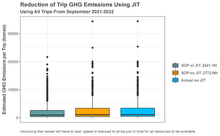
Figure 5: Reduction of trip GHG using JIT. Note: Black line in middle of box corresponds to the median. Black points correspond to outliers (e.g., less than or greater than 95% of the interquartile range)
Comparison of GHG Estimates for Trips using Combinations of SOP and JIT
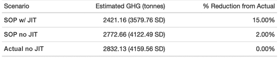
Table 1: Average estimated GHG emissions using SOP and JIT. Note that standard deviations (SD) are quite large due to outlying trips with long durations. Our findings were replicated even when these outliers were removed
Model Validation and Results
As an example case of vessels whose wait times were reduced in comparing the historic to the SOP result, we looked at three trips conducted by a single vessel (“The Vessel”) to a large port on the East Coast of North America (“The Port”) during September 2021-2022. We computed the actual and simulated wait times for these trips. The average actual wait time was 9.58 hours whereas the average simulated wait time was 1.37 hours. In subsequent meetings with Shipping Line representatives, the data and analysis were discussed which led to several key takeaways about the validity of the current analysis as well as practical use of the SOP for reducing GHG emissions.
First, time spent at anchor may not be due to delays or lack of resources at the port. In December 2021, The Vessel spent approximately 20 hours at anchor before berthing. It was revealed by the Shipping Line that this delay was caused by ice buildup on the vessel that needed removing before entering the port. In our analysis, any wait time at anchor was assumed to be due to inefficiencies in the schedule that could be optimized; however, this was clearly a case of a vessel being unable to berth at the time of arrival. While this specific scenario would not necessarily yield improvements due to more efficient resource allocation, there are still potential reductions to GHGs that can be achieved by optimizing speeds due to known delays, in order to reduce wait times. Real-time collaboration and communication of ice buildup may have presented an opportunity to optimize speed given the circumstances. Understanding why vessels are waiting at anchor (or are delayed at berth) would provide a more accurate picture of true wait time as it is conceptualized in the SOP.
Second, current incentives for vessels are not always consistent with optimizing efficiency and JIT. For example, container ships may make more money arriving quickly and waiting at anchor even if it costs more in fuel. Although this highlights an important practical concern for how likely vessels are to follow the SOP and JIT solution, it does not cast doubt on the validity of the solution itself. Indeed, the incoming CII and EEXI regulations from the International Maritime Organization (IMO) may further increase the incentive for vessels to adhere to JIT.
Taken together, the focus on trips and subsequent discussion with the Shipping Line provided concrete methods into how the SOP may be operated in real life scenarios. It demonstrates the importance of obtaining information about the reason for wait times and the consideration of practical and contractual concerns.